2.1. Nonnegative Least Squares Regression¶

Nonnegative Least Squares Regression solves the equation \(Ax=b\) subject to the constraint that the coefficients \(x\) be nonnegative:

\[\underset{x}{\text{argmin}} \quad \| Ax - b \|_2^2, \quad \text{subject to} \quad x \geq 0\]

NonnegativeLinear will take in its fit method arrays X, y and will store the coefficients \(w\) in its coef_ member:

>>> from mcmodels.regressors import NonnegativeLinear
>>> reg = NonnegativeLinear()
>>> reg.fit ([[0, 0], [1, 1], [2, 2]], [0, 1, 2])
NonnegativeLinear()
>>> reg.coef_
array([1.0, 0.0]

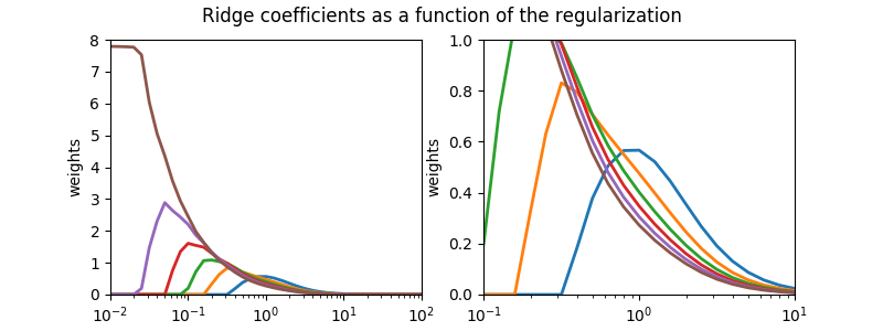
2.1.1. Nonnegative Ridge Regression¶

The equation \(Ax=b\) is said to be ill-conditioned if the columns of A are nearly linearly dependent. Ill-conditioned least squares problems are highly sensitive to random errors and produce estimations with high variance as a result.

We can improve the conditioning of \(Ax=b\) by imposing a penalty on the size of the coefficients \(x\). Using the L2 norm as a measure of size, we arrive at Tikhonov Regularization, also known as ridge regression:

\[\underset{x}{\text{argmin}} \| Ax - b \|_2^2 + \alpha^2 \| x \|_2^2\]

We can incorporate a nonnegativity constraint and rewrite the formula above as a quadratic programming (QP) problem:

(1)¶\[\begin{split}&\underset{x}{\text{argmin}} \quad \| Ax - b \|_2^2 + \alpha^2 \| x \|_2^2 &\quad \text{s.t.} \quad x \geq 0\\ &\underset{x}{\text{argmin}} \quad (Ax - b)^T(Ax - b) + \alpha^2 (x^T I x) &\quad \text{s.t.} \quad x \geq 0\\ &\underset{x}{\text{argmin}} \quad x^TA^TAx - 2b^TAx + b^Tb + x^T \alpha^2 I x &\quad \text{s.t.} \quad x \geq 0\\ &\underset{x}{\text{argmin}} \quad x^TA^TAx + x^T \alpha^2 I x - 2b^TAx &\quad \text{s.t.} \quad x \geq 0\\ &\underset{x}{\text{argmin}} \quad x^T( A^TA + \alpha^2 I )x + (- 2b^TA )x &\quad \text{s.t.} \quad x \geq 0\\ &\underset{x}{\text{argmin}} \quad x^TQx - c^Tx &\quad \text{s.t.} \quad x \geq 0\end{split}\]

where

\[Q = X^TX + \alpha^2 I \quad \text{and} \quad c = - 2A^Ty\]

which we can solve using any number of quadratic programming solvers.

\[\underset{x}{\text{argmin}} \quad x^T(A^TA + \alpha^2 I)x + (-2A^Tb)^Tx \quad \text{s.t.} \quad x \geq 0\]

../_images/sphx_glr_plot_nonnegative_ridge_path_0011.png

As with NonnegativeLinear, NonnegativeRidge will take in its fit method arrays X, y and will store the coefficients \(w\) in its coef_ member:

>>> from mcmodels.regressors import NonnegativeRidge
>>> reg = NonnegativeRidge(alpha=1.0)
>>> reg.fit ([[0, 0], [1, 1], [2, 2]], [0, 1, 2])
NonnegativeRidge(alpha=1.0, solver='SLSQP')
>>> reg.coef_
array([0.45454545, 0.45454545])

2.1.2. Nonnegative Lasso or Nonnegative Elastic Net¶

Both the non-negative Lasso and the non-negative Elastic Net regressors are currently implemented in the scikit-learn package:

If one wishes to perform non-negative Lasso regression, see sklearn.linear_model.Lasso or sklearn.linear_model.lasso_path and pass the parameters fit_intercept=False, positive=True
If one wishes to perform non-negative Elastic-Net regression, see sklearn.linear_model.ElasticNet, or sklearn.linear_model.enet_path, and pass the parameters fit_intercept=False, positive=True

Examples