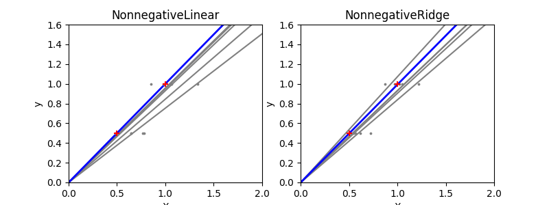
NonnegativeLinear Least Squares and NonnegativeRidge Regression Variance

Note

This example is a copy of plot_ols_ridge_variance.py by Gael Varoquaux and Jaques Grobler in the package Scikit-learn, using NonnegativeLinear and NonnegativeRidge.

Due to the few points in each dimension and the straight line that linear regression uses to follow these points as well as it can, noise on the observations will cause great variance as shown in the first plot. Every line’s slope can vary quite a bit for each prediction due to the noise induced in the observations.

Ridge regression is basically minimizing a penalised version of the least-squared function. The penalising shrinks the value of the regression coefficients. Despite the few data points in each dimension, the slope of the prediction is much more stable and the variance in the line itself is greatly reduced, in comparison to that of the standard linear regression

Out:

# Authors: Joseph Knox <josephk@alleninstitute.org>
# License: Allen Institute Software License

# NOTE: modified from plot_ols_ridge_variance.py by Gael Varoquaux and Jaques Grobler
#       from the package Scikit-Learn licensed under the 3 clause BSD License
#       reproduced below:
#
# New BSD License
#
# Copyright (c) 2007–2018 The scikit-learn developers.
# All rights reserved.
#
#
# Redistribution and use in source and binary forms, with or without
# modification, are permitted provided that the following conditions are met:
#
#   a. Redistributions of source code must retain the above copyright notice,
#      this list of conditions and the following disclaimer.
#   b. Redistributions in binary form must reproduce the above copyright
#      notice, this list of conditions and the following disclaimer in the
#      documentation and/or other materials provided with the distribution.
#   c. Neither the name of the Scikit-learn Developers  nor the names of
#      its contributors may be used to endorse or promote products
#      derived from this software without specific prior written
#      permission.
#
#
# THIS SOFTWARE IS PROVIDED BY THE COPYRIGHT HOLDERS AND CONTRIBUTORS "AS IS"
# AND ANY EXPRESS OR IMPLIED WARRANTIES, INCLUDING, BUT NOT LIMITED TO, THE
# IMPLIED WARRANTIES OF MERCHANTABILITY AND FITNESS FOR A PARTICULAR PURPOSE
# ARE DISCLAIMED. IN NO EVENT SHALL THE REGENTS OR CONTRIBUTORS BE LIABLE FOR
# ANY DIRECT, INDIRECT, INCIDENTAL, SPECIAL, EXEMPLARY, OR CONSEQUENTIAL
# DAMAGES (INCLUDING, BUT NOT LIMITED TO, PROCUREMENT OF SUBSTITUTE GOODS OR
# SERVICES; LOSS OF USE, DATA, OR PROFITS; OR BUSINESS INTERRUPTION) HOWEVER
# CAUSED AND ON ANY THEORY OF LIABILITY, WHETHER IN CONTRACT, STRICT
# LIABILITY, OR TORT (INCLUDING NEGLIGENCE OR OTHERWISE) ARISING IN ANY WAY
# OUT OF THE USE OF THIS SOFTWARE, EVEN IF ADVISED OF THE POSSIBILITY OF SUCH
# DAMAGE.


from __future__ import print_function

import numpy as np
import matplotlib.pyplot as plt

from mcmodels.regressors import NonnegativeLinear, NonnegativeRidge


print(__doc__)

n_datasets = 5

X_train = np.c_[.5, 1].T
y_train = [.5, 1]
X_test = np.c_[0, 2].T

np.random.seed(0)

regressors = dict(NonnegativeLinear=NonnegativeLinear(),
                  NonnegativeRidge=NonnegativeRidge(alpha=0.1))

fig, axes = plt.subplots(1, 2, figsize=(8, 3))

for ax, (name, reg) in zip(axes, regressors.items()):

    for _ in range(n_datasets):
        this_X = .15 * np.random.normal(size=(2, 1)) + X_train
        reg.fit(this_X, y_train)

        ax.plot(X_test, reg.predict(X_test), color='.5')
        ax.scatter(this_X, y_train, s=3, c='.5', marker='o', zorder=10)

    reg.fit(X_train, y_train)
    ax.plot(X_test, reg.predict(X_test), linewidth=2, color='blue')
    ax.scatter(X_train, y_train, s=30, c='r', marker='+', zorder=10)

    ax.set_xlim(0, 2)
    ax.set_ylim((0, 1.6))

    ax.set_xlabel('X')
    ax.set_ylabel('y')

    ax.set_title(name)

plt.show()